This post continues the data exploration started in the previous blog post. Here we will look deeper into the TEP ‘faultless’ dataset in order to better understand it.

Grouping the sensor readings

We previously loaded the dataset, renamed it with more descriptive variable names and explained the meaning of the ‘sample’, ‘simulationRun’ and ‘fault’ columns. Now we will look at the default values of each variable and see how they change over time for each simulation run. Since we are dealing with 52 different variables (not accounting for the 3 previous ones that were already explained), it is advisable to try to categorize them into different groups to make the data more manageable. We can group the columns as follows:

• Pressure (separator, reactor and stripper)
• Level (separator, reactor and stripper)
• Temperature (separator, reactor and stripper, reactor cooling water out and condenser cooling water out)
• Composition of reactor feed (4 feed components, 1 byproduct and 1 inert)
• Composition of product stream (2 feed components, both products and 1 by-product)
• Composition of purge stream (all 8 components)
• Flowrates (A, D and E feed streams, total reactor feed, fresh feed into stripper, recycle flow into reactor, purge rate, underflow of stripper and separator and amount of steam going into the stripper).
• Valves (egulate the flow of the process streams as required)
• Miscallaneous (in this case, only the work done by the compressor).

Understanding the variables

Let’s briefly talk about each group listed above. The pressure, temperature and level variables are naturally used to monitor some of the key process units (in this case the seperator, reactor and stripper). The reactor has a cooling jacket to control the temperature and as such has a tag that monitors the exit temperature of the cooling water. Similarily, the condensor uses cooling water to lower the temperature of the hot stream and thus also montors the exit temperature of the cooling water.

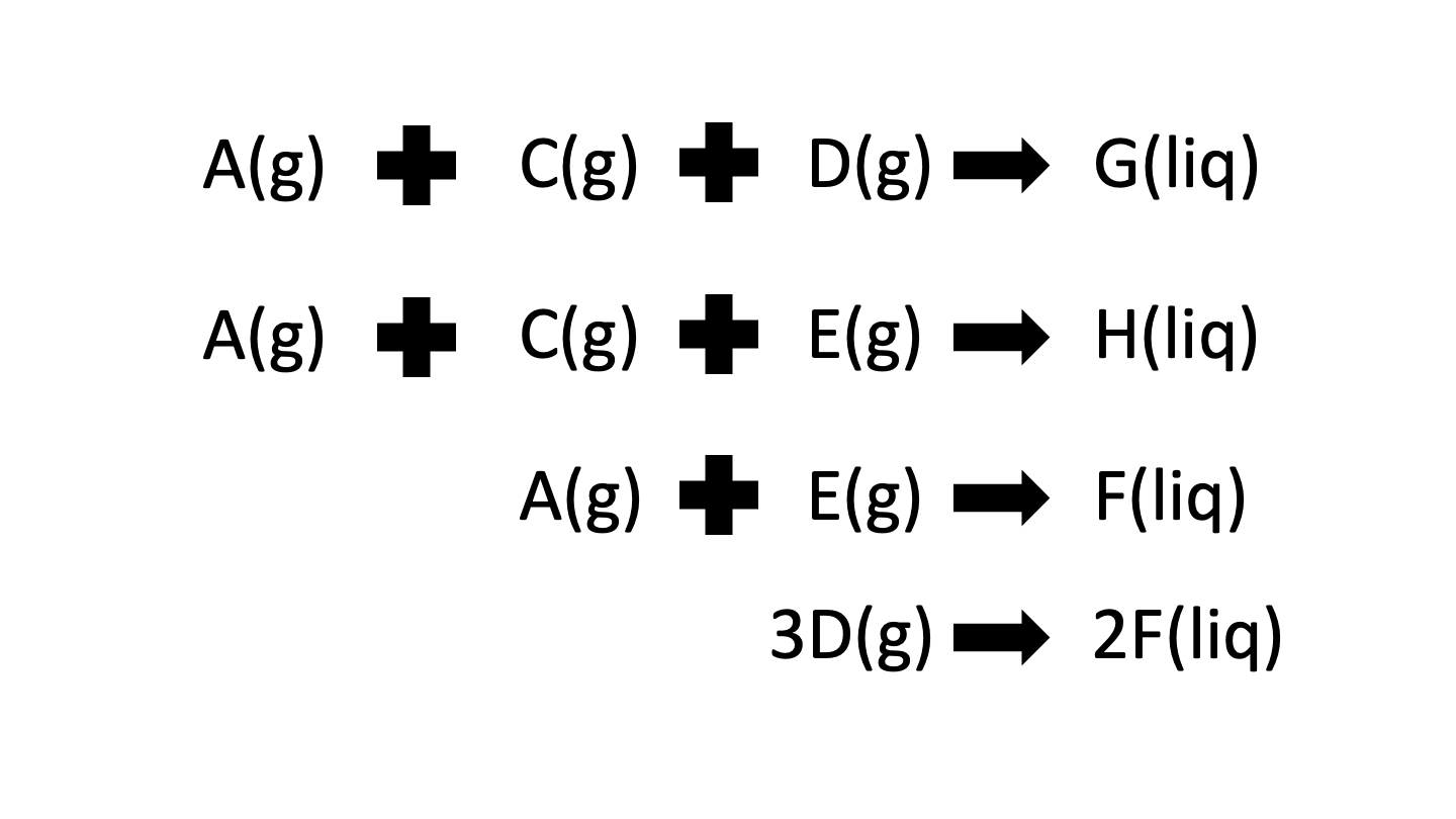
The composition of 3 main streams is continuously monitored in the TEP: the feed into the reactor, the product stream coming out of the stripper and the purge stream. In total there are 8 components at play in this process; 4 reactants (A, C, D and E), 2 products (G and H), 1 by-product (F) and 1 inert (B) as per the reaction scheme given below. It is clear that the separation of products from reactants is assumed to be almost perfect as there are no product components that have been recorded. On the otherhand, all 8 components are monitored in the purge stream to ensure that no valuable products are excessively lost. Lastly, the product stream records the presence of both products, 1 by-product and 2 of the 4 feed components.

A number of flowrates of the TEP are measured such as the feeds and exits of the main process units. These flowrates can sometimes be controlled by the operator by adjusting different valves. Lastly, there is one miscellaneous tag in the dataset which corresponds to the work done by the compressor.

Exploring the data

Now finally to the fun part! Let’s take a variable, in this case it will be the reactor pressure, and see how it changes over time for simulationRun 1. As we can see in the image below, it seems that the pressure oscillates in a Gaussian fashion around a mean value.

df[df['simulationRun']==1]['Reactor_pressure'].plot()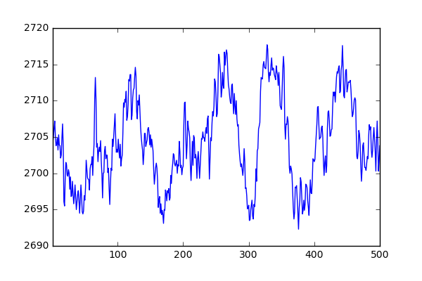

In fact, the same is true for all the simulations that make up this dataset. Below we select 10 random simulationRuns and plot the reactor pressure. It can be seen that not only do they follow the same pattern as before, but their mean and standard deviations are very close to one another.

import random
# For random selection of simulation runs, plot a chosen variable
for run in random.sample(range(1,500),5):
    tmp = df[df['simulationRun']==run].reset_index()
    item = 'Reactor_pressure'
    
    tmp[item].plot()
    print(tmp[item].mean(), tmp[item].std())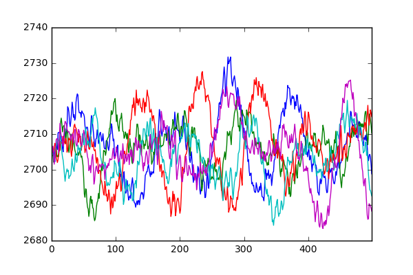

A quick look through the rest of the dataset shows that the other variables behave in a similar fashion to the one see above. Why is this the case? Well it seems that the dataset is highlighting only one normal state of operation for the TEP and is simulating the noise that you would typically find in sensor readings. Each sensor has its own level of accuracy and therefore some tags have a smaller amount of noise than others. This level of noise essentially determines the detection threshold of your anomaly detection method (i.e. it has to be outside the sensor noise level to avoid flagging up too many false positives).

Seperating anomalies from noise

Let’s try the following approach. We can check if the distribution of the pressure follows a normal distribution by doing a quantile-quantile plot. If we get a relatively straight line, then the distribution can be said to be normal.

from statsmodels.graphics.gofplots import qqplot
qqplot(df['Reactor_pressure'].values)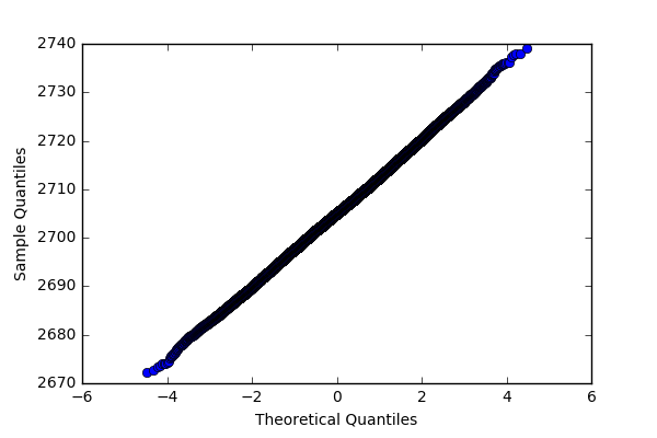

Given that we know that the distribution is normal, we can estimate the population properties: mean and standard deviation. If we want to have a 99% confidence in whether a certain value should be considered an anomaly, we simply check if the value is less than MEAN - 2.58 x STD or if the value is more than MEAN + 2.58 x STD. So for the reactor pressure, the value should be more than 2724.5 or less than 2685.6 for it to be considered an anomaly. Using this same approach, the mean and 2.58 x STD of each variable is listed below:

• A_feed_stream : 0.25 +- 0.08
• D_feed_stream : 3663.79 +- 87.74
• E_feed_stream : 4508.82 +- 101.18
• Total_fresh_feed_stripper : 9.35 +- 0.22
• Recycle_flow_into_rxtr : 26.9 +- 0.55
• Reactor_feed_rate : 42.34 +- 0.56
• Reactor_pressure : 2705.04 +- 19.42
• Reactor_level : 75.0 +- 1.4
• Reactor_temp : 120.4 +- 0.05
• Purge_rate : 0.34 +- 0.03
• Separator_temp : 80.11 +- 0.62
• Separator_level : 50.0 +- 2.6
• Separator_pressure : 2633.77 +- 20.29
• Separator_underflow : 25.16 +- 2.62
• Stripper_level : 50.0 +- 2.62
• Stripper_pressure : 3102.23 +- 16.82
• Stripper_underflow : 22.95 +- 1.59
• Stripper_temperature : 65.8 +- 1.1
• Stripper_steam_flow : 232.16 +- 26.73
• Compressor_work : 341.43 +- 4.26
• Reactor_cooling_water_outlet_temp : 94.6 +- 0.34
• Condenser_cooling_water_outlet_temp : 77.29 +- 0.67
• Composition_of_A_rxtr_feed : 32.19 +- 0.75
• Composition_of_B_rxtr_feed : 8.89 +- 0.27
• Composition_of_C_rxtr_feed : 26.38 +- 0.81
• Composition_of_D_rxtr_feed : 6.88 +- 0.28
• Composition_of_E_rxtr_feed : 18.78 +- 0.76
• Composition_of_F_rxtr_feed : 1.66 +- 0.07
• Composition_of_A_purge : 32.96 +- 0.87
• Composition_of_B_purge : 13.82 +- 0.28
• Composition_of_C_purge : 23.98 +- 1.0
• Composition_of_D_purge : 1.26 +- 0.26
• Composition_of_E_purge : 18.58 +- 0.86
• Composition_of_F_purge : 2.26 +- 0.07
• Composition_of_G_purge : 4.84 +- 0.17
• Composition_of_H_purge : 2.3 +- 0.14
• Composition_of_D_product : 0.02 +- 0.03
• Composition_of_E_product : 0.84 +- 0.05
• Composition_of_F_product : 0.1 +- 0.03
• Composition_of_G_product : 53.73 +- 1.3
• Composition_of_H_product : 43.83 +- 1.3
• D_feed_flow_valve : 63.05 +- 1.51
• E_feed_flow_valve : 53.97 +- 1.21
• A_feed_flow_valve : 24.64 +- 7.84
• Total_feed_flow_stripper_valve : 61.3 +- 3.21
• Compressor_recycle_valve : 22.22 +- 1.37
• Purge_valve : 40.06 +- 3.94
• Separator_pot_liquid_flow_valve : 38.1 +- 7.65
• Stripper_liquid_product_flow_valve : 46.53 +- 6.07
• Stripper_steam_valve : 47.96 +- 7.01
• Reactor_cooling_water_flow_valve : 41.1 +- 1.4
• Condenser_cooling_water_flow_valve : 18.12 +- 3.78

One thing that becomes immediately apparent from this dataset is that it fails to represent the real transience that occurs in recorded operating data. For instance, there are no large spikes in sensor values that occur when a sensor fails. Furthermore, this dataset captures only one normal operating state whereas in reality, there may be many others.

In the next blog post, we will look at the TEP ‘faulty’ dataset to see how it is different to the ‘faultless’ dataset explored here.