In my 2 previous posts, I performed some data exploration on the TEP faultless dataset. We found data that contained simulated sensor readings of 52 features describing the behaviour of Tennessee Eastman process during normal operation (whilst also accounting for stochastic variations). This data was then used to determine the upper and lower detection limits of the reactor pressure which can then be applied to catch potential faults.
In this post, we will look at the TEP faulty dataset that simulates the behaviour of these same process variables but with the substantial difference that the ‘faultNumber’ column now contains values from 1 to 20. This value refers to the introduction of a specific fault in the system after 1 hour of normal operation.
Exploring the Dataset
The TEP faulty dataset is loaded in the same way as the previous faultless dataset. Doing a quick analysis of this dataset, we see that we have 154 different simulation runs (corresponding to different random number generator states) each of which simulates the 20 different faults. Each simulation of a fault has 500 different samples with each sample corresponding to a 3 minute timestep. This means that each simulation lasts for 25 hours and that in total we have a dataset with 500 samples x 154 simulations x 20 faults = 1.54 million entries.
Each value in the ‘fault’ corresponds to a particular deviation from normal operation as caused by the set of faults listed in the table below (taken from this source):
| Fault ID | Description | Type |
|---|---|---|
| 1 | A/C Feed ratio, B Composition constant | Step |
| 2 | B Composition, A/C Ratio constant | Step |
| 3 | D Feed temperature | Step |
| 4 | Reactor cooling water inlet temperature | Step |
| 5 | Condenser cooling water inlet temperature | Step |
| 6 | A Feed loss | Step |
| 7 | C Header pressure loss – reduced availability | Step |
| 8 | A, B, C Feed composition | Random variation |
| 9 | D Feed temperature | Random variation |
| 10 | C Feed temperature | Random variation |
| 11 | Reactor cooling water inlet temperature | Random variation |
| 12 | Condenser cooling water inlet temperature | Random variation |
| 13 | Reaction kinetics | Slow drift |
| 14 | Reactor cooling water valve | Sticking |
| 15 | Condenser cooling water valve | Sticking |
| 16 | Unknown | Random variation |
| 17 | Unknown | Random variation |
| 18 | Unknown | Step |
| 19 | Unknown | Random variation |
| 20 | Unknown | Random variation |
From this table, we can see that there is a good variety of different failures. There are faults related to sticking valves, natural variation in the feed conditions and step changes in certain parameters. Interestingly, there are 5 faults whose origin is deliberatley left unknown; this is done to really challenge our anomaly detection method so that we don’t cheat and tailor our algorithm too much to the dataset.
Finding Fault #1
Now let’s look at how some of the process variables change over time for different faults. We saw that for normal operation, all process variables would oscillate around their means with a normal distribution, each with a distinct standard deviation. Let’s see for instance how fault 1 affects the reaction pressure for 10 different simulations.
for run in random.sample(range(1,184),10):
    tmp = df[(df['simulationRun']==run)&(df['faultNumber']==1)].reset_index()
    item = 'Reactor_pressure'

    fig = tmp[item].plot()

UPPER_LIMIT = 2724.5
LOWER_LIMIT = 2685.6

plt.plot([20,20],[2600,2850],'-r')
plt.plot([0,500],[UPPER_LIMIT,UPPER_LIMIT],'-k')
plt.plot([0,500],[LOWER_LIMIT,LOWER_LIMIT],'-k')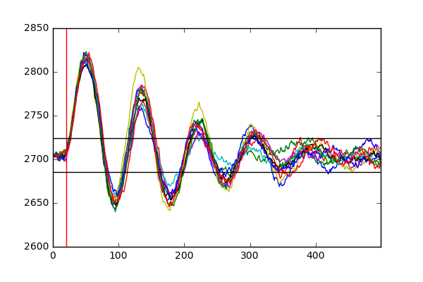
We can clearly see that there is a significant amount of variation in the reactor pressure for this dataset as opposed to the previous one. Each simulation suggests that the introduction of this disturbance in the system causes large swings in the pressure which decay over time. We can also see that the upper and lower detection limits that we derived last time catch the occurrence of this fault shortly after it has been introduced (after 1 hour, or 20 samples) with the system gradually returning to a steady equilibrium after around 350 samples. Zooming into the first 100 samples, we can see how quickly upper and lower limits on the pressure pick up the occurence of the fault:
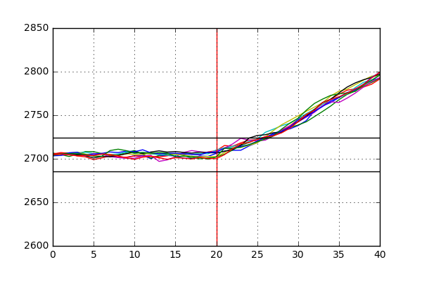
The detection window ranges from around 4 to 7 samples (corresponding to 12-21 minutes) after the introduction of the fault.
Finding Fault #3
Let’s try this technique for another fault, in this case fault 3.
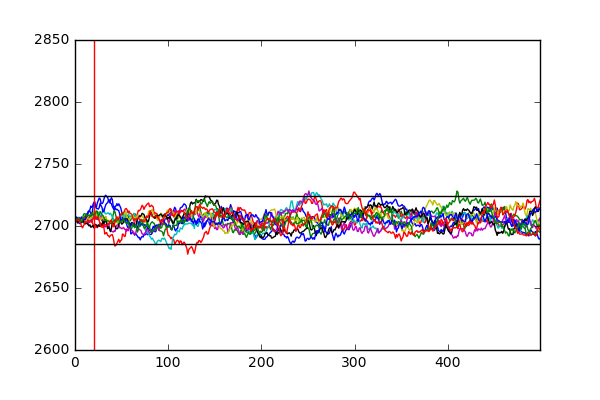
The introduction of fault 3 causes no substantial change in the reactor pressure and thus cannot be picked up by our approach of relying on value thresholds to signal a fault. However, potentially the substantial deviation of another value that might be more susceptible to the, in this case, change in the feed temperature of component D might be able to pick up this fault. Another important point from this exercise, is to see that while that sometimes it might be trivial to pick up a fault, it is not trivial to find out its cause. In this case, while we can pick up the occurrence of fault 2 by catching the increase in the reactor pressure, it does not state what caused it occur. A good anomaly detection algorithm would be also able to find the root cause of the detected fault, in this case a change in the composition of the component B. This relates more to the problem of fault propagation and has been tackled in the literature (I would recommend this source for a good primer).
What’s Next?
Hopefully, from the last 3 posts you have gained an appreciation and understanding of the TEP dataset and its use in anomaly detection. For future posts, I will be using this dataset to test old and new algorithms alike employed for fault detection to showcase both their strengths and weaknesses. Until next time!